In Excel, the VLookup function searches for value in the left-most column of table_array and returns the value in the same row based on the index_number.
The syntax for the VLookup function is:
VLookup( value, table_array, index_number, not_exact_match )
value is the value to search for in the first column of the table_array.
table_array is two or more columns of data that is sorted in ascending order.
index_number is the column number in table_array from which the matching value must be returned. The first column is 1.
not_exact_match determines if you are looking for an exact match based on value. Enter FALSE to find an exact match. Enter TRUE to find an approximate match, which means that if an exact match if not found, then the VLookup function will look for the next largest value that is less than value.
Note:
If index_number is less than 1, the VLookup function will return #VALUE!.
If index_number is greater than the number of columns in table_array, the VLookup function will return #REF!.
If you enter FALSE for the not_exact_match parameter and no exact match is found, then the VLookup function will return #N/A.
Applies To:
- Excel 2007, Excel 2003, Excel XP, Excel 2000
For example:
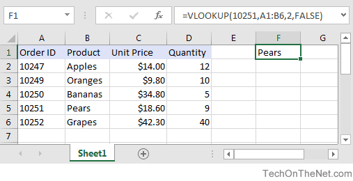
Let's take a look at an example:

Based on the Excel spreadsheet above:
=VLookup(10251, A1:B21, 2, FALSE) would return "Tofu" =VLookup(10251, A1:C21, 3, FALSE) would return $18.60 =VLookup(10248, A1:B21, 2, FALSE) would return #N/A =VLookup(10248, A1:B21, 2, TRUE) would return "Queso Cabrales"
Frequently Asked Questions
Question: In Excel, I'm using the VLookup function to return a value. I want to sum the results of the VLookup, but I can't because the VLookup returns a #N/A error if no match is found. How can I sum the results when there are instances of #N/A in it?
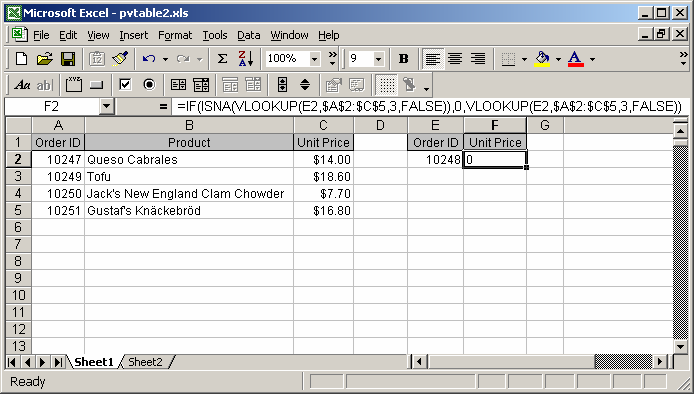
Answer: To perform mathematical operations on your VLookup results, you need to replace the #N/A error with a 0 value (or something similar). This can be done with a formula that utilizes a combination of the VLookup function, IF function, and ISNA function.

Based on the spreadsheet above:
would return
First, you need to enter a FALSE in the last parameter of the VLookup function. This will ensure that the VLookup will test for an exact match.
If the VLookup function does not find an exact match, it will return the #N/A error. By using the IF and ISNA functions, you can return the Unit Price value if an exact match is found. Otherwise, a 0 value is returned. This allows you to perform mathematical operations on your VLookup results.
Question: I have a list of #s in column A (lets say 1-20). There is a master list in another column that may not include some of the column A #s. I want a formula in column B to say (if A1 exists in the master list, then "Yes", "No"). Is this possible?
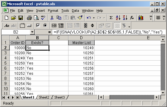
Answer: This can be done with a formula that utilizes a combination of the VLookup function, IF function, and ISNA function.

Based on the spreadsheet above:
=IF(ISNA(VLOOKUP(A2,$D$2:$D$185,1,FALSE)),"No","Yes")
would return "No"=IF(ISNA(VLOOKUP(A5,$D$2:$D$185,1,FALSE)),"No","Yes")
would return "Yes"
First, you need to enter a FALSE in the last parameter of the VLookup function. This will ensure that the VLookup will test for an exact match.
If the VLookup function does not find an exact match, it will return the #N/A error. By using the IF and ISNA functions, you can return a "Yes" value if an exact match is found. Otherwise, a "No" value is returned.
Question: Is there a simple way in Excel to VLookup the second match in a column? So, for instance, If I had apple, pear, apple listed in the column (each word in a separate cell), would there be a way to look up the values to the right of the second "apple"?
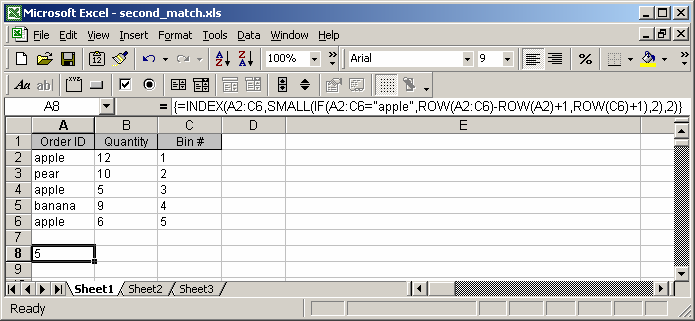
Answer: This can be done with a formula that utilizes a combination of the Index function, Small function, Row function (all in an array formula).

If you wanted to return the quantity value for the second occurrence of apple, you would use the following array formula:
=INDEX(A2:C6,SMALL(IF(A2:C6="apple",ROW(A2:C6)-ROW(A2)+1,ROW(C6)+1),2),2)
When creating your array formula, you need to use Ctrl+Shift+Enter instead of Enter. This creates {} brackets around your formula as follows:
{=INDEX(A2:C6,SMALL(IF(A2:C6="apple",ROW(A2:C6)-ROW(A2)+1,ROW(C6)+1),2),2)}
If you wanted to return the quantity value for the third occurrence of apple, you would use the following array formula:
=INDEX(A2:C6,SMALL(IF(A2:C6="apple",ROW(A2:C6)-ROW(A2)+1,ROW(C6)+1),3),2)
When creating your array formula, you need to use Ctrl+Shift+Enter instead of Enter. This creates {} brackets around your formula as follows:
{=INDEX(A2:C6,SMALL(IF(A2:C6="apple",ROW(A2:C6)-ROW(A2)+1,ROW(C6)+1),3),2)}
If you wanted to return the bin # for the second occurrence of apple, you would use the following array formula:
=INDEX(A2:C6,SMALL(IF(A2:C6="apple",ROW(A2:C6)-ROW(A2)+1,ROW(C6)+1),2),3)
When creating your array formula, you need to use Ctrl+Shift+Enter instead of Enter. This creates {} brackets around your formula as follows:
{=INDEX(A2:C6,SMALL(IF(A2:C6="apple",ROW(A2:C6)-ROW(A2)+1,ROW(C6)+1),2),3)}
If you wanted to return the bin # for the third occurrence of apple, you would use the following array formula:
=INDEX(A2:C6,SMALL(IF(A2:C6="apple",ROW(A2:C6)-ROW(A2)+1,ROW(C6)+1),3),3)
When creating your array formula, you need to use Ctrl+Shift+Enter instead of Enter. This creates {} brackets around your formula as follows:
{=INDEX(A2:C6,SMALL(IF(A2:C6="apple",ROW(A2:C6)-ROW(A2)+1,ROW(C6)+1),3),3)}